To install tensorflow, make sure you have the latest version of pip installed. Type pip install tensorflow at the command line.
The below is a tutorial using code sourced from the following links:
https://www.tensorflow.org/get_started/mnist/beginners https://www.tensorflow.org/get_started/mnist/pros
And information sourced from the Ujjwal Karn's blog:
https://ujjwalkarn.me/2016/08/11/intuitive-explanation-convnets/
All MNIST data can be found at Yann Lecun's website:
from tensorflow.examples.tutorials.mnist import input_data
from __future__ import print_function
import os
import gzip
import numpy as np
import tensorflow as tf
import random
#Define file extraction function
IMAGE_SIZE = 28
NUM_CHANNELS = 1
PIXEL_DEPTH = 255
NUM_LABELS = 10
def extract_data(filename, num_images):
#Extract the images into a 4D tensor [image index, y, x, channels].
#Values are rescaled from [0, 255] down to [-0.5, 0.5].
    print('Extracting', filename)
    with gzip.open(filename) as bytestream:
        bytestream.read(16)
        buf = bytestream.read(IMAGE_SIZE * IMAGE_SIZE * num_images)
        data = np.frombuffer(buf, dtype=np.uint8).astype(np.float32)
        data = data.reshape(num_images, IMAGE_SIZE, IMAGE_SIZE, 1)
    return data

def extract_labels(filename, num_images):
#Extract the labels into a vector of int64 label IDs.
    print('Extracting', filename)
    with gzip.open(filename) as bytestream:
        bytestream.read(8)
        buf = bytestream.read(1 * num_images)
        labels = np.frombuffer(buf, dtype=np.uint8).astype(np.int64)
    return labels

def make_one_hot(labels):
    one_hot_labels = []
    for array in labels:
        hot_vect = [0] * 10
        hot_vect[array] = 1
        one_hot_labels.append(hot_vect)
    one_hot_labels = np.array(one_hot_labels)
    return one_hot_labels

def weight_variable(shape):
    initial = tf.truncated_normal(shape, stddev=0.1)
    return tf.Variable(initial)

def bias_variable(shape):
    initial = tf.constant(0.1, shape=shape)
    return tf.Variable(initial)

def conv2d(x, W):
    return tf.nn.conv2d(x, W, strides=[1, 1, 1, 1], padding='SAME')

def max_pool_2x2(x):
    return tf.nn.max_pool(x, ksize=[1, 2, 2, 1],
                        strides=[1, 2, 2, 1], padding='SAME')
#Load in MNIST training data
train_data_filename = "../tf_tutorial/MNIST_data/train-images-idx3-ubyte.gz"
train_labels_filename = "../tf_tutorial/MNIST_data/train-labels-idx1-ubyte.gz"
test_data_filename = "../tf_tutorial/MNIST_data/t10k-images-idx3-ubyte.gz"
test_labels_filename = "../tf_tutorial/MNIST_data/t10k-labels-idx1-ubyte.gz"

train_data = extract_data(train_data_filename, 55000)
train_labels = extract_labels(train_labels_filename, 55000)
test_data = extract_data(test_data_filename, 10000)
test_labels = extract_labels(test_labels_filename, 10000)
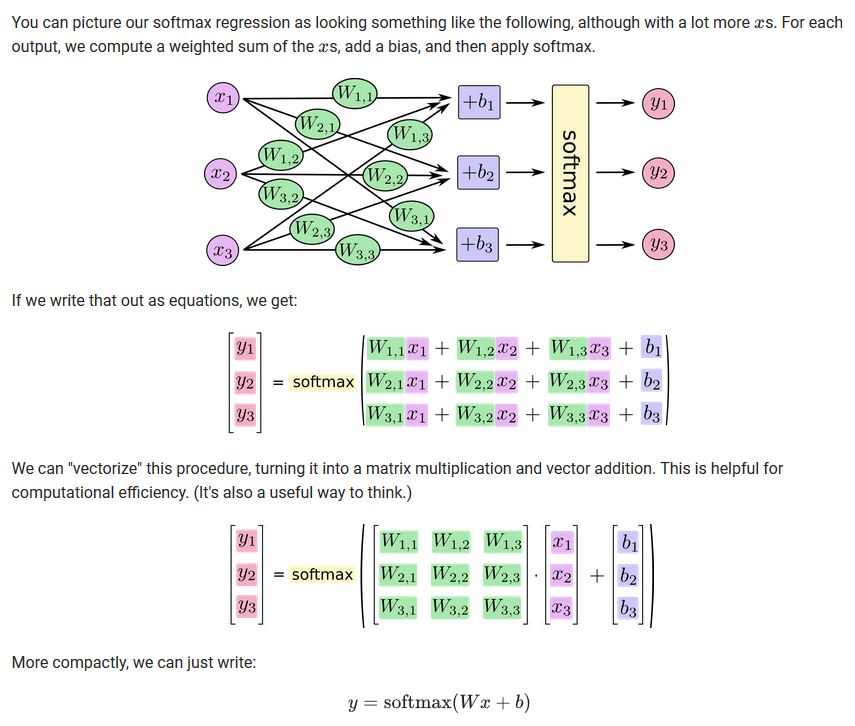
Build out a simple Softmax Neural Network (Logistic Regression)
#Create an interactive tensorflow session
sess = tf.InteractiveSession()

#Set placeholders
x = tf.placeholder(tf.float32, shape=[None, 784])
y_ = tf.placeholder(tf.float32, shape=[None, 10])

#Declare variables
W = tf.Variable(tf.zeros([784,10]))
b = tf.Variable(tf.zeros([10]))

#Run the interactive session
sess.run(tf.global_variables_initializer())

#Create prediction
y = tf.matmul(x,W) + b
#Set the cost function that the NN minimizes
cross_entropy = tf.reduce_mean(
    tf.nn.softmax_cross_entropy_with_logits(labels=y_, logits=y))

#Train the model
train_step = tf.train.GradientDescentOptimizer(0.5).minimize(cross_entropy)
hot_train_labels = make_one_hot(train_labels)
for _ in range(1000):
    batch = random.sample(zip(train_data,hot_train_labels) , 100)
    image_batch = [a for (a,b) in batch]
    image_batch = np.reshape(image_batch, (-1, 784))
    label_batch = [b for (a,b) in batch]
    sess.run(train_step, feed_dict={x: image_batch, y_: label_batch})
#Evaluate the simple softmax model
correct_prediction = tf.equal(tf.argmax(y,1), tf.argmax(y_,1))
accuracy = tf.reduce_mean(tf.cast(correct_prediction, tf.float32))
hot_test_labels = make_one_hot(test_labels)
#Run the empty models above with our train and test data
reshaped_test = np.reshape(test_data, (-1,784))
print(sess.run(accuracy, feed_dict={x: reshaped_test, y_: hot_test_labels}))
Convolutional Neural Network
#The image needs to be a 4d tensor
x = tf.placeholder(tf.float32, shape=[None, 28, 28, 1])

#First Convolutional Layer
W_conv1 = weight_variable([5, 5, 1, 32])
b_conv1 = bias_variable([32])
#x_image = tf.reshape(x, [-1, 28, 28, 1])
h_conv1 = tf.nn.relu(conv2d(x, W_conv1) + b_conv1)
h_pool1 = max_pool_2x2(h_conv1)

#Second Convolutional Layer
W_conv2 = weight_variable([5, 5, 32, 64])
b_conv2 = bias_variable([64])
h_conv2 = tf.nn.relu(conv2d(h_pool1, W_conv2) + b_conv2)
h_pool2 = max_pool_2x2(h_conv2)

#Densely Connected Layer
W_fc1 = weight_variable([7 * 7 * 64, 1024])
b_fc1 = bias_variable([1024])
h_pool2_flat = tf.reshape(h_pool2, [-1, 7*7*64])
h_fc1 = tf.nn.relu(tf.matmul(h_pool2_flat, W_fc1) + b_fc1)

#Dropout - note that dropout is a technique to deal with overfitting.
#The general idea is too randomly drop units (along with their connections) from the NN during training.
keep_prob = tf.placeholder(tf.float32)
h_fc1_drop = tf.nn.dropout(h_fc1, keep_prob)

#Readout layer, this is simply the last layer in the network and combines the results from the second layer
W_fc2 = weight_variable([1024, 10])
b_fc2 = bias_variable([10])
y_conv = tf.matmul(h_fc1_drop, W_fc2) + b_fc2
#Train and evaluate the model
cross_entropy = tf.reduce_mean(
    tf.nn.softmax_cross_entropy_with_logits(labels=y_, logits=y_conv))
train_step = tf.train.AdamOptimizer(1e-4).minimize(cross_entropy)
correct_prediction = tf.equal(tf.argmax(y_conv, 1), tf.argmax(y_, 1))
accuracy = tf.reduce_mean(tf.cast(correct_prediction, tf.float32))
hot_train_labels = make_one_hot(train_labels)
hot_test_labels = make_one_hot(test_labels)

with tf.Session() as sess:
    sess.run(tf.global_variables_initializer())
    for i in range(10000):
        batch = random.sample(zip(train_data,hot_train_labels), 50)
        image_batch = [a for (a,b) in batch]
        label_batch = [b for (a,b) in batch]
        if i % 1000 == 0:
            train_accuracy = accuracy.eval(feed_dict={x: image_batch, y_: label_batch, keep_prob: 1.0})
            print('step %d, training accuracy %g' % (i, train_accuracy))
        train_step.run(feed_dict={x: image_batch, y_: label_batch, keep_prob: 0.5})

    print('test accuracy %g' % accuracy.eval(feed_dict={x: test_data, y_: hot_test_labels, keep_prob: 1.0}))
So what's going on exactly?
First, convince yourself that every image can be represented as a matrix of numeric values.
![]()
We use the term channel to refer to the different dimensions that an image can take. For example, consider a color photograph. If we are only considering the colors, then each color takes on a value for each of three channels: red, green, and blue. This is represented by three stacked 2-dimensional matrices, each having numeric values in the range 0 to 255.
Let us define a convolution operator:
$(f*g)(t) = \int_{0}^{t} f(\tau) g(t-\tau)d \tau \text{ for } f,g: [0, \infty]$
In the context of a CNN, our convolutions are dot products across different subsection of the input matrix and a filter matrix. The different subsections of the input matrix are determined by stride size. Let's do an example below.
Consider the following input matrix:
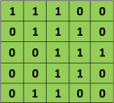
Let the filter matrix be:

Set the stride size to be one so that we slide over the input matrix by 1 pixel for each convolution. We generate a 3x3 matrix from the input matrix starting at element [1,1], then we create another 3x3 matrix starting at the point [1,2]. We keep iterating until we can no-longer create clean 3x3 matrix subsets of the input matrix. This occurs at element [3,3]. Visually, our convolution looks like:
We're left with a 3x3 matrix that we call the Convolved Feature/Activation Map/Feature Map.
Different filters will result in different feature maps. See below for a quick example using a picture of a squirrel:
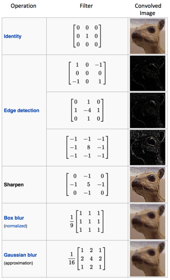
In practice, a CNN learns the values of these filters during the training process. The hyper parameters that we specify in learning include the number of filters, filter size, and architecture of the network (number of layers).
Filter size is controlled by three hyper-parameters:
- Depth: The number of filters we use, this determines the number of feature maps.
- Stride: The number of pixels by which we slide the filter matrix over the input matrix.
- Zero-padding: Whether or not to pad the outside edges of the input matrix with zeros. We do this because when we slide the filter matrix over the input matrix, we might not pick up a matching subset matrix size without going over the boundaries of the input matrix.
Rectifier function in a CNN (ReLU)
Note that ReLU stands for Rectified Linear Unit. It is defined as: $f(x) = max(0,x)$
This has the following graph:
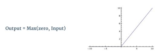
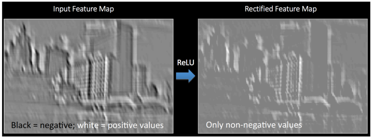
The rectifier works by replacing all negative pixel values in the feature map (result of the convolution) by zero. In this sense it is an element-wise operation. We do this to introduce non-linearity into our ConvNet (otherwise a simple dot product is just a linear transformation). See below for an example of ReLU being applied to an image:
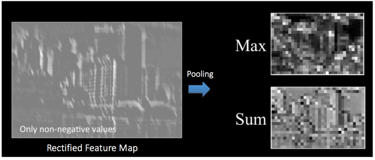
Pooling
There are different types of pooling: average, max, mode, sum, etc. But it's a method by which to pool together the outputs of a neural network layer.
Max pooling works by the following algorithm:
- Define a spatial neighborhood (say 2x2 window)
- Choose a stride size (same idea as above but we apply it to the feature map)
- Take the largest element from the rectified feature map within the window
- Generate a reduced dimensionality of the feature map, this is called the output map
See below for an example of max and sum pooling being applied to the rectified feature map above:
A major advantage of pooling is that it makes the overal neural network invariant to small transformations. That is, if we suddenly see a large outlier in one of our pixel elements it won't have an outsized impact on the network because it's being pooled with all the other pixel elements.
Fully Connected Layer
This is the final layer in the neural network. This is a traditional multi layer perceptron and it acts as a classifier for the features generated by the convolution and pooling layers. The popular choice is a softmax function but other classifiers such as SVM can be used as well.
For more on multilayer perceptrons see:
https://ujjwalkarn.me/2016/08/09/quick-intro-neural-networks/
The term fully connected implies that every neuron in the previous layer is connected to every neuron on the next layer. We use a fully connected to layer to learn a non-linear combination of these features. The result of this layer is a classification probability for each class (if softmax is used).
Backpropagation
The training of a CNN has the following algorithm:
- Initialize all filters/parameters/weights with random values
- Pick a training image. Use this as an input to the network and forward propagate the network:
- Convolute the image
- Apply ReLU/Pooling operations
- Classify using the fully connected layer
- Calculate the total error at the output layer:
$Total Error = \frac{1}{2}\sum (target probability - output probability)^{2}$
- Use Backpropagation to calculate the gradients (derivative) of the total error w.r.t all weights in the network. Use gradient descent to update all filters/parameters/weight values to minimize the output error.
- Repeat steps 2-4 with all images in the training set
The above steps make it such that the CNN has been optimized to correctly classify images from the training set. The idea is that, given a big enough training set that is representative of the "true" distribution of images, the trained model shold be able to do a good job at classifying images that it has yet to see.