Latent Dirichlet Allocation (LDA)

LDA models each document as a mixture over topics. Each topic is a distribution over a selection of words and each word within the corpus of docuemnts is assumed to be from a particular distribution of words. The algorithm takes the number of topics, $k$, as a parameter. Each $k$ is called a latent topic. LDA produces the support for each topic distribution via Bayesian updating. In general LDA:

• Starts with each document being represented as a bag of words.
• Produces the word distribution for each topic using approximating methods
• Returns a vector of length $k$ for each document, where each entry is the weight per distribution for each document

On a high level, we are interested in solving the following conditional probability:

$ p(\theta, \textbf{z} | \textbf{w}, \alpha, \beta) = \frac{p(\theta, \textbf{z}, \textbf{w}| \alpha, \beta)} {p(\textbf{w}| \alpha, \beta)} $

Where:

$ \theta \text{ is a parameter drawn from a Dirichlet distrubtion characterized by }\alpha \\ \textbf{z} \text{ is a vector of topics, where each z is drawn from a multinomial distrubtion characterized by } \theta \\ \textbf{w} \text{ is a vector of words such that each $w$ has multinomial probability $p(w|z, \beta)$} $

Note that $\alpha$ and $\beta$ are user-specified parameters. Unfortunately, the above conditional probabilty does not have a closed form solution and we must use approximating methods to find a solution. Below is an outline for a popular method.

Collapsed Gibbs Sampling

1. Go through each document D, and randomly assign each word in D to one of the $k$ topics.

2. For each D, go through each word W in D, and for each topic $k$:

   1. Compute P($k$|D) = The probability of a topic given a document. This is the proportion of words in document D that are currently assigned to topic T
   2. Compute P(W|$k$) = The probability of a word given a topic. This is the proportion of document assignments to topic T over all documents that result from the word W.

1. Assign W to a new topic. We choose the new topic by computing the probability P($k$|D) x P(W|$k$) for each topic and then pick the topic with the highest probability. This is the probability that topic T generated word W, holding everything else constant. In this step, we're assuming that all topic assignments except for the current word are correct, and then updating the assignment of the current word using our model of how documents are generated.
2. Repeat steps 2 and 3 until we reach a rough steady state. That is, the support of the distribution of topic T (the underlying words in the distribution) are not changing more than some minimal threshold.

After generating the topics, we can represent each document as a weight from each topic. Recall that we already represent the document as a bag of words, so we essentially combine the word counts for words in the same latent topic when we compute topic weights. That is, we compute the topic mixtures of each document by counting the proportion of words assigned to each topic within that document.

See here for an application of this methodology in Spark

Word2Vec

These are models first devloped by Mikolov et al (2013) which use the physical closeness of words to derive context. In general, these models use a 2-layer neural network to produce a vector space for a given corpus such that each vector in the space (one for each unique word) is "close" to other vectors that share similiar meaning.

There are two main neural network structures for this idea: the continuous bag of words model and the skip-gram model. The continuous bag of words model predicts the current word given the surrounding words. The skip-gram model predicts the surrounding words given the current word.

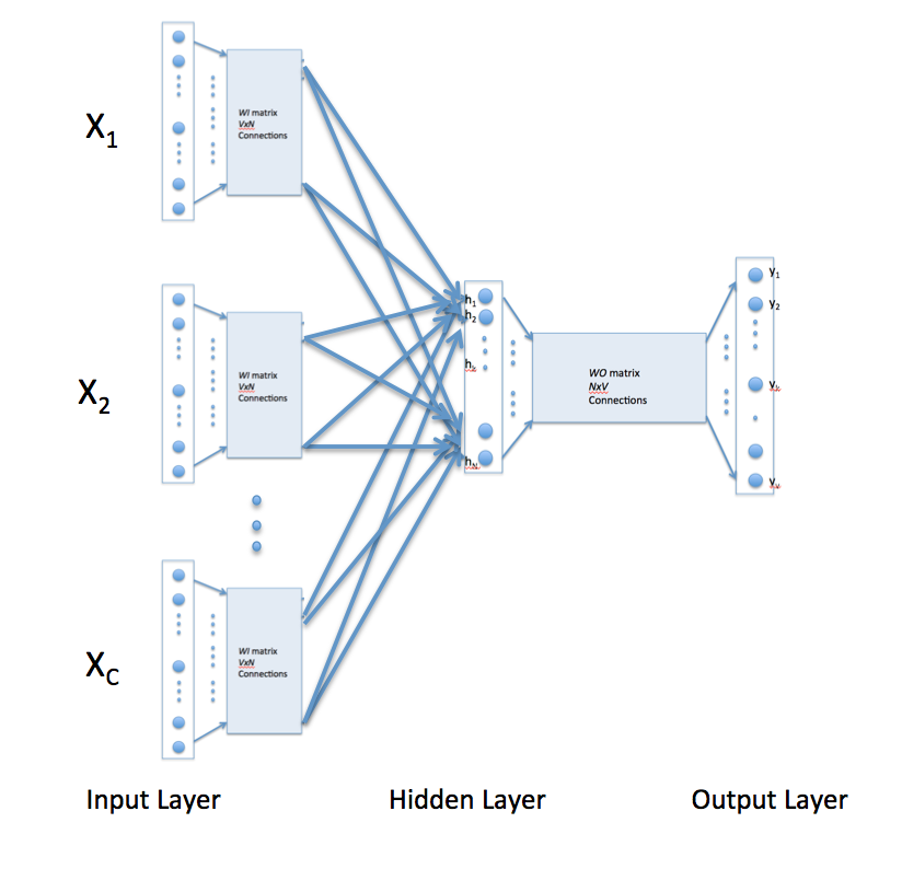
The above describes a continuous bag of word neural network model, the image is taken from this blog post

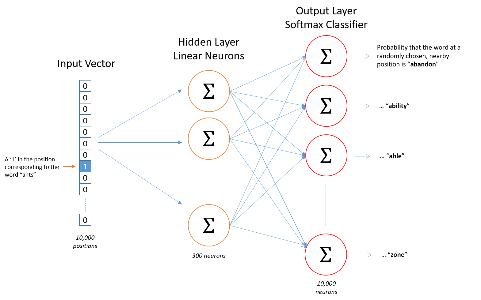
The above describes a skip-gram neural network model, the image is taken from this blog post

The result from both of these models is a vector for each word that contains the surrounding words most related in semantic meaning. That is, it returns a vector of words that are most correlated with a given word. We can think of these vectors as "topics" in the sense that a vector for a given topic will contain words most related to that topic.

Some issues with this is approach:

1. Back-propagation in a two-layer neural network means that the results are a black box
2. The model is highly sensitive to the corpus that it is trained on, meaning any changes to the data cleaning process will be reflected in the model results
3. Language is non-stationary, the authors use a Word2Vec model on the entire corpus of 10-Ks. It is not clear that this is appropriate (especially given the difficulty in parsing 10-K documents prior to 2005)

For more information see the wikipedia link and the original paper

Latent Semantic Analysis (LSA)

LSA is a dimensionality reduction tool for bag of word models. The LSA algorithm takes a term-document matrix and performs a singular value decomposition. Then, it selects a subset of eigen-values, K, and performs a rank K approximation of the original term-document matrix. K is a parameter and is commonly referred as the number of "topics".

LSA assumes that the physical closeness of words imply the same concept. For example, the word bank when close to the words mortgage, interest rate, or loan is conceptually related to a financial institution whereas if the word bank shows up next to lures, casting, and fish probably implies a stream or river bank. The expectation is that the lower dimensional representation merges together the dimensions associated with terms that have similar meanings.

For more information, see:

https://en.wikipedia.org/wiki/Latent_semantic_analysis

Derivation

Let $X$ be a term-document matrix where the rows are the terms and the columns are the documents in the corpus, so that each document is represented as a word count of different terms.

By singular value decomposition, there exists a decomposition of $X$ such that $X = U E V'$, where $U$ and $V$ are orthogonal matrices and $E$ is a diagonal matrix.

We have that:

$XX' = U E V'V E' U' = UE^{2}U'$

$X'X = V E' U'U E V' = VE^{2}V'$

Note that $E$ is diagonal, so that both $XX'$ and $X'X$ have the same eigenvalues. Further, $U$ must contain the eigenvectors of $XX'$ and $V$ must contain the eigenvectors of $X'X$. We can interpret $V$ as containing the "document" eigenvectors while $U$ contains the "term" eigenvectors.

import io
import base64
from IPython.display import HTML

video = io.open('topic_model_scheme.webm', 'r+b').read()
encoded = base64.b64encode(video)
HTML(data='''<video alt="test" controls>
                <source src="data:video/mp4;base64,{0}" type="video/mp4" />
             </video>'''.format(encoded.decode('ascii')))

Selecting $k$ largest singular values (the square root of the elements of $E'E$) and their corresponding eigenvectors in $V$ and $U$ leads to the rank $k$ approximation of $X$.

We refer to $k$ as the number of topics. The term eigenvector that each $k$ eigenvalue is associated with is the particular mix of terms that make up each topic.

Click here for more information